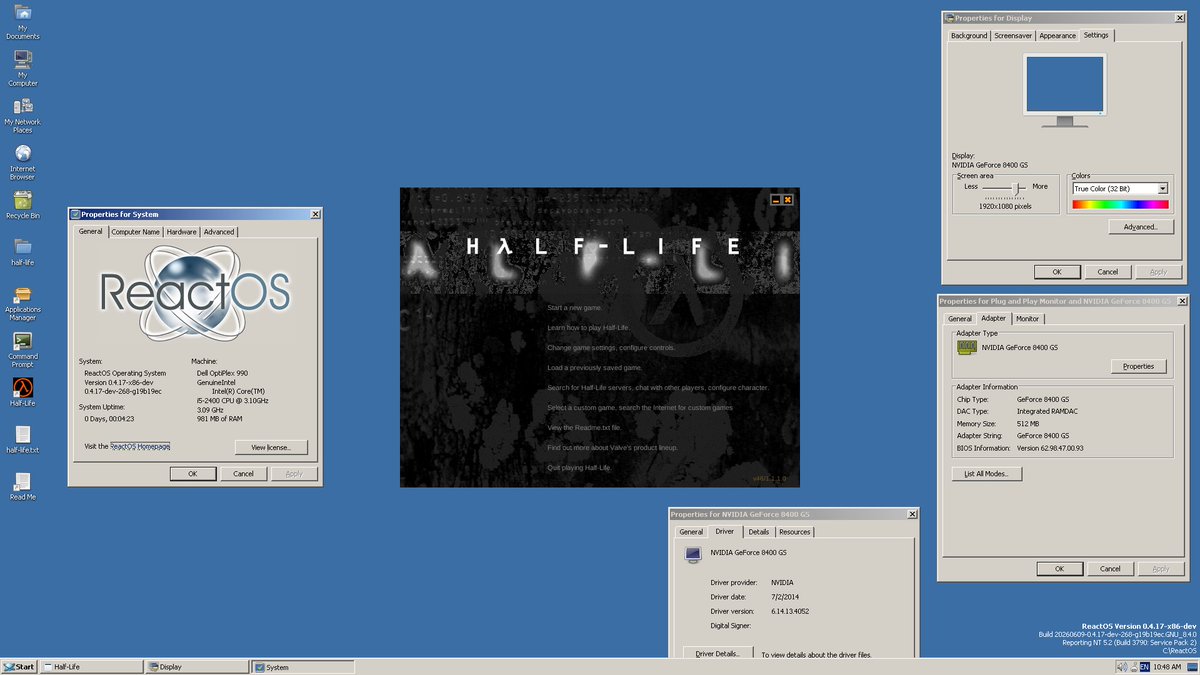
Here's Half-Life with #ReactOS - see the hardware it runs on!! Courtesy of Zombiedeth.

AI is using AI to use AI to do my job! What do I do now?

0 classifications 0 Set A (probe) 0 Set B (solver) — solver calls avoided Theoretical Result A 6.36σ universal separability signal exists across the SAT phase transition — a previously undescribed structural property of random k-SAT, validated n=15 to n=500 on random 3-SAT · SATLIB benchmarks n=50–100. This signal partitions instances without solver invocation, enabling 57% solver call reduction on hard phase-transition instances. Parks SAT Framework (PTSF) · Alika M. Parks · Kalaheo, Hawaii · 2026 — instances classified globally Performance Metrics 57% solver call reduction · Tier 1 classifier 47x vs MiniSAT · Tier 1 · benchmark hardware · n=50 3.9x vs Kissat · Tier 2 VIG-CDCL solver · mean n=20–100 9.7x vs Kissat · Tier 2 peak · n=75 6.36σ universal separability signal · n=15 to n=500 0.999 Tier 1 accuracy · SATLIB validated 100% Tier 2 solver correctness · n=20–100 validated Tier 1 (classifier): ~57% · no solver ·

Open-source NVMe sanitization framework with 50 cycles and per-cycle Log Page 0x81 hardware confirmation. PDF Certificate of Destruction. Designed to align with NIST SP 800-88 Rev.2. Free. - yonasa...

Verifiable digital identities and secure login for AI agents. One API call. No redirects.

A Danish computer, GIER, from 1961 played a vital role in the development of a new method for astrometric measurement. This method, photon counting astrometry, ultimately led to two satellites with a significant role in the modern revolution of astronomy. A GIER was installed at the Hamburg Observatory in 1964 where it was used to implement the entirely new method for the measurement of stellar positions by means of a meridian circle, then the fundamental instrument of astrometry. An expedition to Perth in Western Australia with the instrument and the computer was a success. This method was also implemented in space in the first ever astrometric satellite Hipparcos launched by ESA in 1989. The Hipparcos results published in 1997 revolutionized astrometry with an impact in all branches of astronomy from the solar system and stellar structure to cosmic distances and the dynamics of the Milky Way. In turn, the results paved the way for a successor, the one million times more powerful Gaia astrometry satellite launched by ESA in 2013. Preparations for a Gaia successor in twenty years are making progress.

ClawMoat is the agent seatbelt, runtime security for desktop AI agents running on your real machine.

Big Kahuna

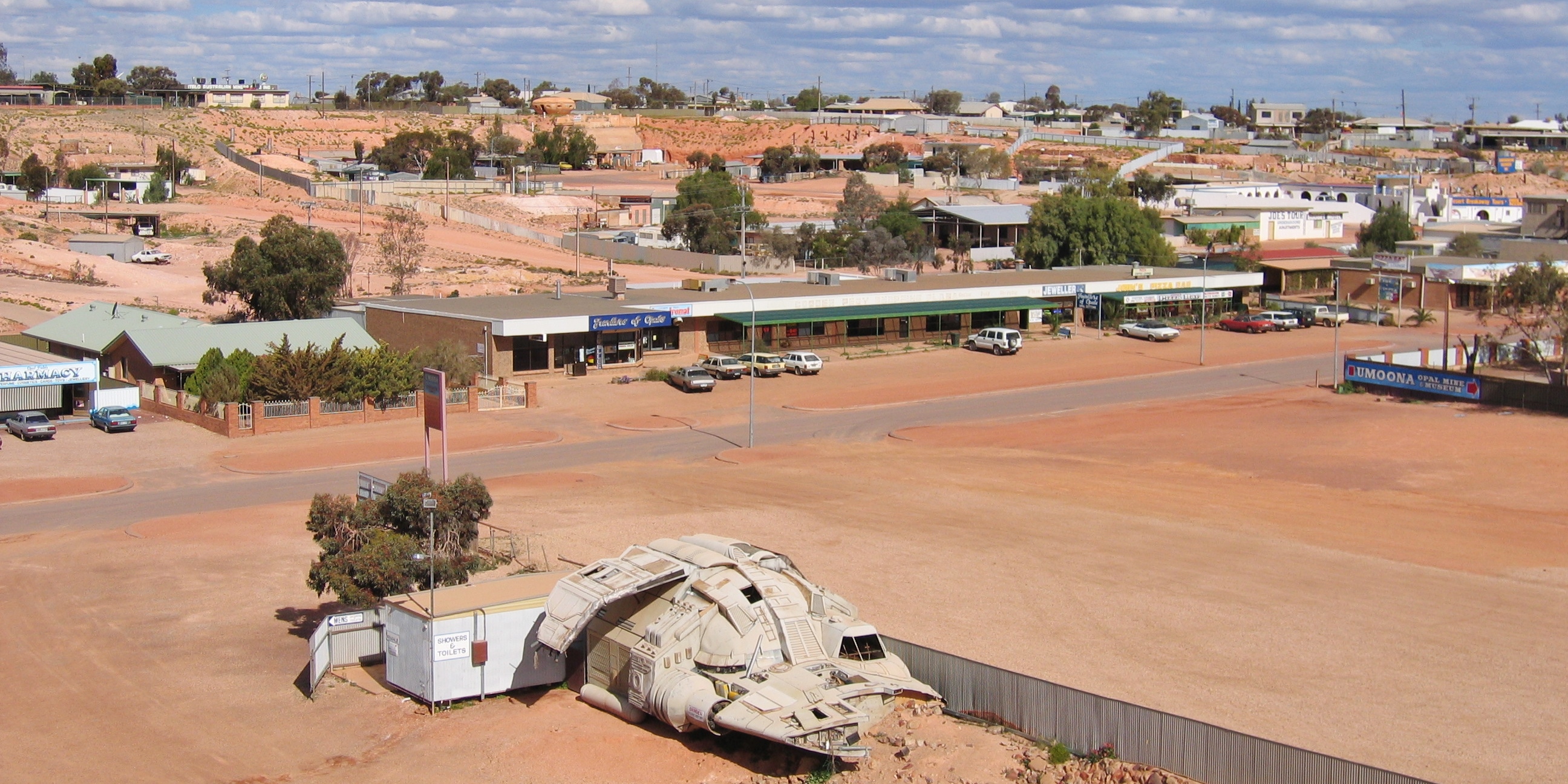
Surface temperatures in Coober Pedy regularly hit 45 °C. So more than half its residents live in cool, climate-stable houses — and even a church and a hotel — carved straight into the sandstone hills.

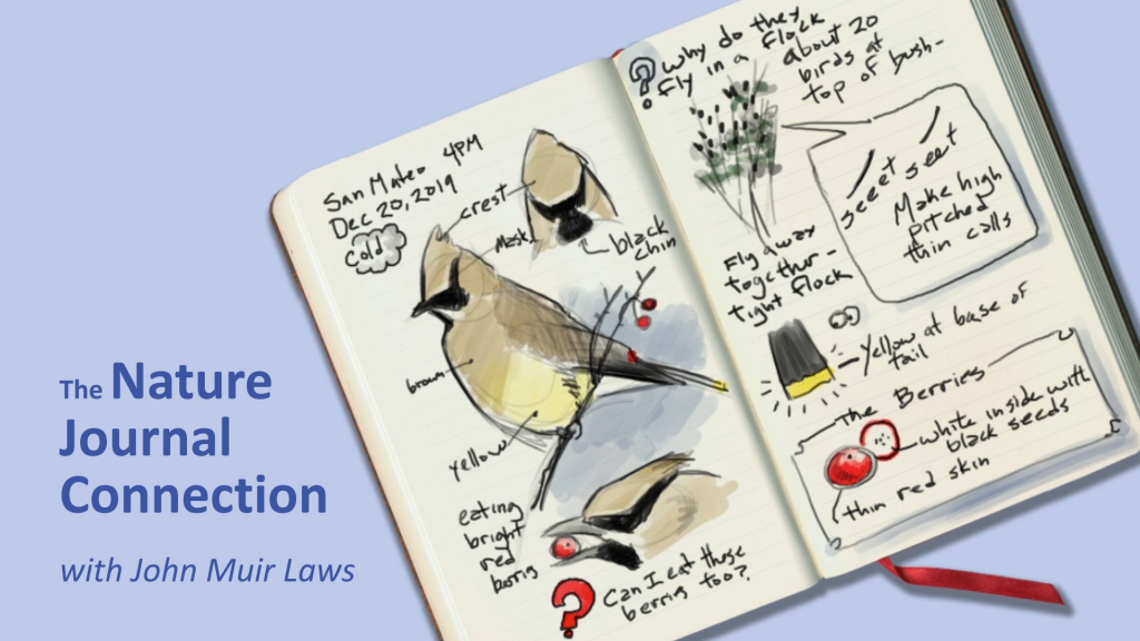
01inspiration I love nature journaling. Over time I've developed a style and approach that I like for capturing sketches quickly, using a Pilot G2 pen in combination with a waterbrush. This lets me add linework and shading simultaneously (I dual wield with the brush in my left hand) and forces me not to be too precious about the final result - there will inevitably be smudges and imperfections, and there is no undo with pen! This project began as a test of Anthropic's new model Claude Fable 5, and grew once I saw the potential to actually recreate that experience in a browser. I love the final result! Example sketches from my notebooks, from fast flamingo figure-drawings to more finessed fan-art fun. Of course, I'm left in a rather funny position: I've 'created' this app, but I haven't actually touched the code! I can read it (it's a rather nice, self-contained single HTML file) since I have experience with the underlying technologies. But I'm hoping that this app is interesting to many people who *aren't* webGL nerds, and so for the sake of all of our collective understanding I've had Fable spin up some interactive demos to illustrate the concepts. You are also welcome to check out the prompts I used to conjure this app into being. Disclaimer: While I've tidied up a bit, the rest of this article contains plenty of AI-witten prose. I don't like AI writing as a rule, especially undisclosed! Hopefully you can forgive me in this case, since (with some iteration) the AI actually did a pretty good job showing all the key pieces. Over time I might refactor and reorganise it to be more in line with my personal sensibilities, but no promises :) 02three sheets of state Under the canvas, the painting is not pixels — it’s a small stack of floating-point textures, ping-ponged through about a dozen WebGL2 fragment shaders every frame. Think of them as transparent sheets laid over each other: fieldformatresolutionmeaning inkRGBA16Fup to 2048, matches screen mobile pigment. RGB is optical density (how much each light channel is absorbed), not color. Alpha is white gouache. fixedRGBA16Fsame as ink pigment that has settled into the paper and no longer moves (section 07). wetR16Fsame as ink how much water is sitting on each point of the paper. velocityRG16F~256 cells on the short side the water’s motion. Coarse on purpose — flow is smooth, pigment is not. pressureR16Fsame as velocity scratch space for keeping the flow incompressible. Each frame: the stroke engine stamps gaussian splats into these fields (section 05), the simulation advances them (03–04), and a final display shader turns density into paper-and-ink color (08). Nothing in the pipeline ever stores “a color” — color only exists for the one shader that draws the screen. You can see the sheets directly. The demo below paints a stroke and washes through it; the buttons switch which field you’re looking at. fig 2An x-ray of the engine. painting is the composed result; pigment is raw ink density; water is the wetness field (note how it spreads past the brush and slowly evaporates); flow shows velocity, direction as hue. The flow only exists where the paper is wet. The two resolutions matter. Velocity lives on a coarse ~256-cell grid because fluid motion is inherently smooth, and the pressure solve (the expensive part) scales with cell count. Pigment and wetness live at up to 2048 — near screen resolution — because that’s where edges, granulation and fine linework live. The sleight of hand of the whole app is sampling a blurry, cheap flow field to push around a sharp, expensive ink field. 03water that moves The flow is Jos Stam’s Stable Fluids (1999), the algorithm behind nearly every realtime smoke, ink and fire toy on the GPU. It earns the “stable” in its name from one idea: don’t push, pull. A naive simulation moves each parcel of fluid forward along its velocity — and explodes the moment a parcel overshoots a grid cell. Stam’s semi-Lagrangian advection flips the question. Each grid cell asks: if the fluid here arrived from somewhere, where was it one timestep ago? It traces backward along the velocity, samples the old field at that point (bilinearly, between the four nearest cells), and adopts the value. No overshoot is possible, because every cell ends up with a weighted average of values that already existed. Big timestep, lazy frame rate, doesn’t matter — it cannot blow up. fig 3Semi-Lagrangian advection. The highlighted cell traces backward along the local velocity (dashed), samples the field between the four nearest cells, and carries that value home. Every cell does this, every frame, in one fragment shader. In GLSL the whole maneuver is two lines: vec2 coord = vUv - uDt * texture(uVelocity, vUv).xy * uTexel; vec2 vel = texture(uVelocity, coord).xy * uDissipation; Advection alone gives you syrup, not water. Two more passes give it character: Pressure projection makes the water incompressible. After advection the velocity field has places where flow piles up (positive divergence) or tears apart (negative). A real liquid refuses both — push it and it must go around. The solver computes the divergence, relaxes a pressure field against it with ~22 Jacobi iterations, and subtracts the pressure gradient from the velocity. What that buys, visibly, is swirl: pushes turn into eddies and curls instead of sprays. Vorticity confinement fights numerical mush. All that bilinear sampling acts like a low-pass filter — little whirlpools blur away within seconds. So the solver measures the curl that remains, finds its ridges, and applies a small force that spins them back up. It’s a knob for liveliness: inkwash ties it (along with the push strength and how slowly velocity decays) to the flow slider. flow · low flow · high fig 4The same scripted strokes — an ink blob, then a circling water brush — at the two ends of the flow slider. Low flow is a damp, obedient wash; high flow has momentum, vorticity, and opinions. 04paper that decides A fluid solver on its own makes smoke — everything drifts forever. What makes this feel like paper is that the wetness field acts as a permission system over the whole simulation. Three gates, all reading the same little texture: Velocity is confined to wet paper. After advecting, the velocity is multiplied by smoothstep(0.005, 0.2, wet) — flow simply cannot exist on dry ground. This is why a wash stops at its own boundary instead of smearing across the page. Pigment mobility is earned, not assumed. The ink pass computes mob = smoothstep(0.02, 0.45, wet) and scales both its advection distance and its bleed rate by it. Damp paper lets ink creep; soaked paper lets it run. Bone-dry paper is a museum — the shader returns the old value untouched and the pixel costs almost nothing. Water itself moves reluctantly. The wet field is advected at only 0.6× the flow speed, blurred a little into its neighbors each frame (capillary creep — a puddle’s edge slowly widens), and decays exponentially. The dry slider sets that time constant, from about 2 to about 18 seconds. Drying is what turns a fluid sim into a painting: every wash is a closing window. fig 5A pen line, then water brushed over its left half. Only the wetted half moves — and only until the paper dries. Slide dry and let the loop replay to feel the working window change. Drying in inkwash is honest in one more way: water doesn’t take the pigment with it when it goes. Wherever ink happens to be when its puddle evaporates, that’s where it stays — mid-bloom, mid-streak, mid-swirl. Most of the textures that read as “watercolor” are just the flow field’s last words, frozen. 05making marks Between your hand and the fields sits a small stroke engine, and it draws everything with a single primitive: a gaussian splat — a fuzzy radial stamp, exp(-d²/r²), blended into a field. A pen stroke is a chain of ink splats; a brush stroke is a chain of water splats plus velocity impulses pointing along the motion. The stamps are spaced at 0.6 of the radius so their overlap sums to a smooth ribbon: fig 6Gaussian stamps along a stroke. Each curve is one splat; the line above is their sum, and the strip is how it renders. At the app’s spacing (0.6×r) the seams vanish; drag the slider apart to see the beads a stroke is secretly made of. How the stamps are blended matters as much as their shape. Ink is additive — densities sum, which (as section 08 will make precise) is exactly how real glazes deepen. Water uses MAX blending instead: wetness saturates rather than accumulates, so scrubbing the brush in place makes paper wet, not impossibly flooded. One blend-equation flag, and it’s the difference between a watercolor and a swamp. The hand data feeding those splats gets shaped, too: Pressure and speed set the nib. For the pen, radius and density both grow with stylus pressure and shrink with speed — a fast flick gives a thin, dry line; a slow, heavy drag gives a dark, swelling one. On a trackpad, Force Touch stands in for pressure; with a mouse or finger, the engine fakes pressure from speed (slow ≈ deliberate ≈ heavy), which is wrong in theory and convincing in practice. The cursor is chased, not obeyed. The brush position relaxes toward the pointer exponentially (k = 1 - exp(-14·dt)). That few-millisecond lag is the cheapest line-quality trick in graphics: jitter is absorbed, corners round off, and strokes get the slight follow-through of a real brush. Stillness is a mark. If the pen dwells in place, ink keeps feeding in at a trickle and the spot blooms — pooling, like resting a real nib on damp paper. A dwelling brush gently stirs the water beneath it instead. fig 7The pen’s vocabulary: a slow, pressure-tapered stroke; a fast light one; and a dwell that pools. Try it yourself — with a stylus you get real pressure, with anything else the speed fake. 06black that isn’t black Here is the trick the whole app was built around. Put a drop of water on a line of cheap black ink and watch the edge: the black stays close, but a blue-violet ghost walks out ahead of it. Black inks are dye cocktails, and on wet paper they chromatograph — each dye travels at its own speed. Inkwash gets this almost for free because of a decision from section 02: pigment is stored as per-channel optical density, and the bleed step — which each frame nudges ink toward the average of its neighbors, where wet — runs at a different rate per channel: // red-absorbing dye escapes fastest, blue-absorbing dye drags behind uChroma = vec3(1.0 + 0.85*C, 1.0 + 0.15*C, max(0.25, 1.0 - 0.65*C)); vec4 bleedAmt = clamp(uBleed * (0.25 + 1.3*brush) * mob * vec4(uChroma, 1.05), 0., 0.92); vec4 mixed = mix(advected, neighborhood, bleedAmt); Read that as chemistry: the component that absorbs red light (and therefore looks cyan-blue) diffuses outward fastest; the component that absorbs blue hangs back in the line. A few seconds of this and any wet edge sorts itself into a dark core with a cool halo — no halo is ever drawn, it separates. The color slider is C in that snippet: at 0 the channels move in lockstep and the ink behaves like lamp black; pushed up, the dyes split apart. One more term worth noticing: brush is a gaussian around the brush tip, so bleeding runs ~5× faster right under the bristles. Scrubbing doesn’t just wet the ink — it actively works it loose, which is exactly what scrubbing should do. fig 8Chromatography on demand: an ink blob, then a circling wet brush. bleed sets how fast pigment diffuses where wet; color sets how differently the channels travel — the source of the blue. Both at zero is well-behaved india ink; both high is the cheapest fountain pen cartridge you ever loved. 07pressing fix Real watercolor layers because dried pigment bonds to the paper — you can glaze over yesterday’s wash without reviving it. A single mobile ink field can’t give you that, which is why inkwash keeps two pigment sheets: ink (mobile) and fixed (settled). Pressing fix (or d) runs a 1.2-second settling pass: each frame a fraction of the mobile pigment transfers to the fixed layer, the velocity field is braked hard, and the wetness flash-dries. The painting looks identical before and after — but it has changed state, from liquid to laminate. fig 9Layering. A diagonal is drawn and washed — it smears. fix. A second diagonal is drawn and washed the same way — only the new stroke moves; the first, now part of the paper, holds. The fix button works on your own marks too. White ink is the other half of the layering story, and it’s sneakier than it looks. White gouache rides in the pigment texture’s alpha channel and composites over the dark ink on screen. But paint white over black, fix it, then draw dark on top — physically you’re drawing on a fresh white ground, so the new line must read dark. If white stayed “a layer on top” forever, it would bleach everything drawn after it. So baking white is destructive, the way real gouache is opaque. At fix time, white coverage bleaches the density underneath it — the dark ink it hides is genuinely removed, in transmittance space — and then the white itself dissolves into the paper: // coverage c of white gouache erases what it hides, then becomes paper float c = (1.0 - exp(-2.2 * whiteAmount)) * uSettle; vec3 T = exp(-density); // current transmittance density = -log(clamp(T * (1.0 - c) + c, 1e-4, 1.0)); fig 10Gouache logic: a dark patch is fixed, a white ring is painted over it and fixed — bleaching what it covers — and then a dark stroke crosses everything and reads dark, even over the white. Three states of the same two textures. 08drawing the paper Everything so far has been bookkeeping in density-land. The display shader is where it becomes a painting, and its core is one physical law. Beer–Lambert: light passing through pigment is attenuated exponentially, per channel. vec3 color = paper * exp(-density * uInkStrength); This is why pigment is stored as density. Overlapping strokes add densities, which multiplies transmittances — and an exponential through a slightly tinted absorption spectrum behaves the way paint does: the first pass is a luminous gray, the fourth is a deep charcoal that still leans cool, and nothing ever clips into flat black. Naive alpha-blending, the default in every drawing API, converges on mud instead: fig 11The same overlapping strokes composited two ways. Left, Beer–Lambert (multiplied transmittance — what inkwash does): overlaps deepen and stay chromatic. Right, standard alpha over: overlaps rush toward a flat gray ceiling. Add strokes with the slider. Around that one law, the display pass layers the things that make paper paper — all generated, nothing sampled from an image: Fiber and tooth. Two octaves-apart value noises (an fbm at large scale, a fine one at pixel scale) tint the blank sheet so it’s never a flat hex code. Granulation. A third noise field modulates ink density — but only where pigment is. That’s the speckle real pigments leave as particles settle into the paper’s valleys. Edge darkening. The shader measures the local gradient of density and multiplies absorption by 1 + 1.35·|∇|. In real watercolor, pigment migrates to a drying wash’s boundary and leaves a dark rim — the single most recognizable watercolor signature. Here it’s a cheap screen-space fake of that, and it’s doing an enormous amount of the look. Wet sheen. Wherever the wet field is high, the paper darkens slightly and coolly — so you can see your working window, watch a wash visibly dry, and know where a new stroke will bloom. fig 12The display pass, dissected. The engine paints the same little wash on loop; the checkboxes turn each rendering ingredient off and on. With everything off, you’re looking at the raw simulation — correct, and dead. 09ways to paint with it The instrument has more registers than its two modes suggest. A few that fall out of the physics: line, then wash wet-on-wet white over dark fig 13Three idioms, looping. Left: the journaling classic — linework, then a wash inside it that feathers the fresh lines into blue-haloed shading. Middle: wet the paper first with a clean brush, then touch the pen into the puddle and let it bloom. Right: fix a dark field, then white ink becomes stars. Line, then wash is the native idiom: draw, press d to fix, then brush freely — your shading can’t destroy your drawing, but fresh ink on top still moves. Wet-on-wet inverts the order: lay clean water first, then drop the pen into it; ink hitting a standing puddle blooms outward instead of holding a line. Dry brush against the clock: with the dry slider high, a wash gives you two seconds of movement and then commits — closer to sumi-e than to watercolor. And the brush ink slider quietly turns the water brush into a loaded watercolor brush, for when you want broad pigment without drawing ten thousand pen lines. The input mapping carries the same pen-and-waterbrush metaphor across devices: On iPad, the Apple Pencil draws and your finger is the water brush — no mode switch, just two different things touching the paper, which is the most honest version of the idea. (A side benefit: strokes are single-pointer, so a resting palm is simply ignored.) On a tablet, the stylus barrel button momentarily swaps pen for brush, like flipping a pencil to its eraser. On a Mac trackpad, Force Touch pressure drives line weight. Failing all of that, keys: b pen / brush w white ink d fix c clear s save png f fullscreen · · · 10colophon Inkwash is a single HTML file — under a thousand lines, no dependencies, no build step. It needs WebGL2 and renderable half-float textures (EXT_color_buffer_float), which is everything from roughly 2021 onward. The full pipeline — twelve shader passes including the 22 Jacobi iterations — runs comfortably at 60 fps on a phone, mostly because the expensive solve happens on the coarse grid. This page is the same engine, refactored just enough to run many instances at once: every demo shares one WebGL context and one set of compiled shaders, keeps its own little stack of field textures, renders to a hidden canvas and copies out — so thirteen simulations coexist without tripping the browser’s context limit, and only the ones on screen actually step. There is also a testing trick inherited from the app: load any of these files with ?demo and the scripted strokes run synchronously at startup, so a headless browser can screenshot a finished painting — which is how an AI assistant and I checked our work while building all of this. back to Johno, the human author: I can't help contrast this project with my first foray into artistic generative webGL stuff - a slime mold sim called dotswarm. That project was a lot of fun, but involved multiple nights tearing my hair out fighting obscure shader bugs. This time around I had the idea, spoke to a computer about it, refined it over time as I zeroed in on what I actually wanted, and ended up with one of my favourite pieces of software ever. All it took was some english language chit-chat! And with a few more turns I ended up with this lovely interactive explainer too. Of course, this isn't exactly rocket science - e.g. the fluid sim piece is a well-known and well-used piece of tech at this point. But still - I'm excited to see things get to the point where such wonderous personal software creation is available to so many people. (Well, right now the model that did this is not available to anyone, thanks to the USG slamming it with export controls - but that's temporary). Anyway, definitely go paint with the app. Check out the source code. But also, think through your backlog of ideas for software you wish existed - there's a chance you can make it now. Good luck :) PS: Here are a few of my sketches done over the course of testing. If you make anything, pretty or not, I'd love to see it! Tag me @johnowhitaker on X. Some test drawings from the first ~day of working on this app :)

Browse, search, install, and snapshot Homebrew packages. Full source. MIT licensed. No telemetry, no accounts.

A few weeks ago an ordinary security assessment turned into an incident response whirlwind. It was definitely a first for me, and I was kindly granted permission to outline the events in this blog post. This investigation started scary but turned out be quite fun, and I hope reading it will be informative to you too. I'll be back to posting about my hardware research soon. How it started What hell is this? The NFS Server 2nd malicious binary Further forensics Eureka Moment The GOlang thingy How the kernel got patched? and why not the golang app? What we have so far Q&A How it started Twice a year I am hired to do security assessments for a specific client. We have been working together for several years, and I had a pretty good understanding of their network and what to look for. This time my POC, Klaus, asked me to focus on privacy issues and GDPR compliance. However, he asked me to first look at their cluster of reverse gateways / load balancers: I had some prior knowledge of these gateways, but decided to start by creating my own test environment first. The gateways run a custom Linux stack: basically a monolithic compiled kernel (without any modules), and a static GOlang application on top. The 100+ machines have no internal storage, but rather boot from an external USB media that has the kernel and the application. The GOlang app serves in two capacities: an init replacement and the reverse gateway software. During initialization it mounts /proc, /sys, devfs and so on, then mounts an NFS share hardcoded in the app. The NFS share contains the app's configuration, TLS certificates, blacklist data and a few more. It starts listening on 443, filters incoming communication and passes valid requests on different services in the production segment. I set up a self contained test environment, and spent a day in black box examination. Having found nothing much I suggested we move on to looking at the production network, but Klaus insisted I continue with the gateways. Specifically he wanted to know if I could develop a methodology for testing if an attacker has gained access to the gateways and is trying to access PII (Personally Identifiable Information) from within the decrypted HTTP stream. I couldn't SSH into the host (no SSH), so I figured we will have to add some kind of instrumentation to the GO app. Klaus still insisted I start by looking at the traffic before (red) and after the GW (green), and gave me access to a mirrored port on both sides so I could capture traffic to a standalone laptop he prepared for me and I could access through an LTE modem but was not allowed to upload data from: The problem I faced now was how to find out what HTTPS traffic corresponded to requests with embedded PII. One possible avenue was to try and correlate the encrypted traffic with the decrypted HTTP traffic. This proved impossible using timing alone. However, unspecting the decoded traffic I noticed the GW app adds an 'X-Orig-Connection' with the four-tuple of the TLS connection! Yay! I wrote a small python program to scan the port 80 traffic capture and create a mapping from each four-tuple TLS connection to a boolean - True for connection with PII and False for all others: 10.4.254.254,443,[Redacted],43404,376106847.319,False 10.4.254.254,443,[Redacted],52064,376106856.146,False 10.4.254.254,443,[Redacted],40946,376106856.295,False 10.4.254.254,443,[Redacted],48366,376106856.593,False 10.4.254.254,443,[Redacted],48362,376106856.623,True 10.4.254.254,443,[Redacted],45872,376106856.645,False 10.4.254.254,443,[Redacted],40124,376106856.675,False ... With this in mind I could now extract the data from the PCAPs and do some correlations. After a few long hours getting scapy to actually parse timestamps consistently enough for comparisons, I had a list of connection timing information correlated with PII. A few more fun hours with Excel and I got histogram graphs of time vs count of packets. Everything looked normal for the HTTP traffic, although I expected more of a normal distribution than the power-low type thingy I got. Port 443 initially looked the same, and I got the normal distribution I expected. But when filtering for PII something was seriously wrong. The distribution was skewed and shifted to longer time frames. And there was nothing similar on the port 80 end. My only explanation was that something was wrong with my testing setup (the blue bars) vs. the real live setup (the orange bars). I wrote on our slack channel 'I think my setup is sh*t, can anyone resend me the config files?', but this was already very late at night, and no one responded. Having a slight OCD I couldn’t let this go. To my rescue came another security? feature of the GWs: Thet restarted daily, staggered one by one, with about 10 minutes between hosts. This means that every ten minutes or so one of them would reboot, and thus reload it’s configuration files over NFS. And since I could see the NFS traffic through the port mirror I had access to, I recokoned I could get the production configuration files from the NFS capture (bottom dotted blue line in the diagram before). So to cut a long story short I found the NFS read reply packet, and got the data I need. But … why the hack is eof 77685??? Come on people, its 3:34AM! What's more, the actual data was 77685 bytes, exactly 8192 bytes more then the ‘Read length’. The entropy for that data was pretty uniform, suggesting it was encrypted. The file I had was definitely not encrypted. Histogram of extra 8192 bytes: When I mounted the NFS export myself I got a normal EOF value of 1! What hell is this? Comparing the capture from my testing machine with the one from the port mirror I saw something else weird: For other NFS open requests (on all of my test system captures and for other files in the production system) we get: Spot the difference? The open id: string became open-id:. Was I dealing with some corrupt packet? But the exact same problem reappeared the next time blacklist.db was send over the wire by another GW host. Time to look at the kernel source code: The “open id” string is hardcoded. What's up? After a good night sleep and no beer this time I repeated the experiment and convincing myself I was not hullucinating I decided to compare the source code of the exact kernel version with the kernel binary I got. What I expected to see was this (from nfs4xdr.c): static inline void encode_openhdr(struct xdr_stream *xdr, const struct nfs_openargs *arg) { __be32 *p; /* * opcode 4, seqid 4, share_access 4, share_deny 4, clientid 8, ownerlen 4, * owner 4 = 32 */ encode_nfs4_seqid(xdr, arg->seqid); encode_share_access(xdr, arg->share_access); p = reserve_space(xdr, 36); p = xdr_encode_hyper(p, arg->clientid); *p++ = cpu_to_be32(24); p = xdr_encode_opaque_fixed(p, "open id:", 8); *p++ = cpu_to_be32(arg->server->s_dev); *p++ = cpu_to_be32(arg->id.uniquifier); xdr_encode_hyper(p, arg->id.create_time); } Running binwalk -e -M bzImage I got the internal ELF image, and opened it in IDA. Of course I didn’t have any symbols, but I got nfs4_xdr_enc_open() from /proc/kallsyms, and from there to encode_open() which led me to encode_openhdr(). With some help from hex-rays I got code that looked very similiar, but with one key difference: static inline void encode_openhdr(struct xdr_stream *xdr, const struct nfs_openargs *arg) { ... p = xdr_encode_opaque_fixed(p, unknown_func("open id:", arg), 8); ... } The function unknown_func was pretty long and complicated but eventually sometimes decided to replace the space between 'open' and 'id' with a hyphen. Does the NFS server care? Apparently this string it is some opaque client identifier that is ignored by the NFS server, so no one would see the difference. That is unless they were trying to extract something from an NFS stream, and obviously this was not a likely scenario. OK, back to the weird 'eof' thingy from the NFS server. The NFS Server The server was running the 'NFS-ganesha-3.3' package. This is a very modular user-space NFS server that is implemented as a series of loadable modules called FSALs. For example support for files on the regular filesystem is implemented through a module called libfsalvfs.so. Having verified all the files on disk had the same SHA1 as the distro package, I decided to dump the process memory. I didn't have any tools on the host, so I used GDB which helpfully was already there. Unexpectadly GDB was suddenly killed, the file I specified as output got erased, and the nfs server process restarted. I took the dump again but there was nothing special there! I was pretty suspicious at this time, and wanted to recover the original dump file from the first dump. Fortunately for me I was dumping the file to the laptop, again over NFS. The file had been deleted, but I managed to recover it from the disk on that server. 2nd malicious binary The memory dump was truncated, but had a corrupt version of NFS-ganesha inside. There were two libfsalvfs.so libraries loaded: the original one and an injected SO file with the same name. The injected file was clearly malicious. The main binary was patched in a few places, and the function table into libfsalvfs.so as replaced with the alternate libfsalvfs.so. The alternate file was compiled from NFS-ganesha sources, but modified to include new and improved (wink wink) functionality. The most interesting of the new functionality were two separate implementations of covert channels. The first one we encountered already: When an open request comes in with 'open-id' instead of 'open id', the file handle is marked. This change is opaque to the NFS server, so unpatched servers just ignore it and nothing much happens. For infiltrated NFS server, when the file handle opened this way is read, the NFS server appends the last block with a payload coming from the malware's runtime storage, and the 'eof' on-the-wire value is changed to be the new total size. An unpatched kernel (which shouldn’t really happen, since it…