How does the ML research community feel about evolutionary algorithms? Should I do a PhD in this area? Quick remark: I know some people in the ML community dunk on evolutionary algorithms because there’s often a better optimizer, but they do have their place, which is what researchers in my community aim to quantify. Background: I just finished my first year as a mathematics master’s student working on the theory of evolutionary algorithms (EAs)/randomized search heuristics. I’m fortunate to be on a research assistantship and have already coauthored several papers in strong conferences in our area. I’ve always been more interested in classical ML/deep learning theory but haven’t had anyone to work with. Researchers in my field, including my advisor, occasionally publish in mainstream ML venues such as AAAI and NeurIPS, but it’s primarily the EA venues. For a while now, I’ve been independently studying deep learning and statistical learning theory, and I have found intersections with my current research that I plan to pursue for my thesis. With my current CV, it’s looking like I could get into some of the best PhD programs in my area, but I’m wondering if I should try to go to a more ML-centric PhD, even if it means going to a less prestigious institution/group for the sake of my career. I’m not sure yet what I want to do after my PhD and a possible postdoc, but I want to keep myself competitive for top-tier opportunities. What implications might doing an EA PhD have for my career? With strong EA publications, could I get into a good ML PhD program if I pitch myself appropriately? Could staying somewhat outside mainstream ML actually be a good career move, given how competitive and crowded ML has become? submitted by /u/NullRecurrentDad [link] [Kommentare]

Reviewing ArkType after writing about branded types and parsing in TypeScript. Turns out someone built the thing I was hand-rolling.

"The calculus of relations has an intrinsic charm and beauty which makes it a source of intellectual delight to all who become acquainted with it." —Alfred Tarski Prela is an embedded query language focusing on compositionality and control. Its queries are concise, clear, and fast. It is implemented as a library of query combinators (think parser combinators), allowing the user to freely intermix queries with code in the host programming language. The implementation follows continuation-passing style, resulting in a core engine under 1k lines of code that compiles to efficient columnar execution. Unlike almost all SQL databases, Prela does not come with its query optimizer, and queries are executed exactly as they are written. This gives the user complete control over all aspects of query planning, including join ordering, operator pushdown, materialization, and selection of physical data structures. Nevertheless, the most idiomatic way to write a query already performs well in our experiments. Prela is a research prototype in early development. Expect constant and sweeping changes to both language design and implementation. Intuitively, the query looks for movies satisfying several conditions: Then, for each such movie, output the following attributes: In SQL's way of thinking, movie would be in the FROM clause (along with other tables involved), with corresponds to the WHERE clause,1 and select corresponds to the SELECT clause. But unlike SQL, Prela can freely interleave predicates and outputs, resulting in more natural queries as shown above. You can also think of data.with(...).text() and company.with(...).name() parts as subqueries which require special syntax in SQL, but are just subexpressions in Prela. And instead of explicit conditions, joins in Prela are reflected by the structure of the query in a navigational style. To understand what's going on under the hood, we should first clarify the data model used by Prela. The theoretical foundation of Prela is a formalism of relations 100 years older than the familiar relational algebra, called (confusingly) relation algebra. To avoid confusion, I will call it Tarski's Algebra of Relations (TAR) after the logician responsible for its modern formalization. In TAR (and therefore Prela), everything is a binary relation, and a query is built up with operators that take in and produce binary relations, which I call relation combinators. One way to think about this is a very extreme form of normalization: every table with k columns is "shredded" into k binary tables, one per column. Let us consider a simplified version of the query above: Here, title and production_year are both attributes of the same table in the original schema, but in Prela, each of them becomes a binary relation, mapping every movie (ID) to its title and production year, respectively. movie is also a binary relation, albeit a little special: it corresponds to the primary-key ID column of the original table, and is the identity relation over the IDs; in other words, movie contains (i, i) for every ID i in the table. Overall, each "column table" can be thought of as a map from the primary key to its corresponding value. Comparisons like .gt() and .is_in() are regular Rust methods on relations. For example, production_year.gt(2008) returns a binary relation that's a subset of production_year, such that the second column (the "value" column) contains only values greater than 2008. Next, .with() is the restriction combinator: r.with(s) restricts the last column of the r with the first column of the s; i.e., it is exactly a left-semijoin. In this example, movie.with(production_year.gt(2008)) semijoins movie with the filterd-out production_year relation, and since movie is the identity relation, we're left with the IDs for movies made after 2008. The .select() combinator is relational composition. It is the workhorse of both Prela and TAR. The key to understanding relational composition is to view relations as a generalization of functions: a binary relation of type (X, Y) generalizes a function of type X -> Y by allowing multiple different "output" (Y) values per "input" (X). For this reason, we will abuse X -> Y to denote the type of a binary relation. From this perspective, it is then natural to see select as a generalization of the function composition (\(f \circ g\)): r.select(s) first "applies" r to each x to get a bunch of y, then for each y, apply s to get a bunch of z. In math: \(R \circ S = \lbrace (x, z) \mid \exists y . (x, y) \in R \land (y, z) \in S \rbrace\). In standard relational algebra: \(R \circ S = \pi_{x, z}(R \Join_{R.y = S.y} S)\) where R's schema is over x and y, and S's schema is over y and z. Going back to our example, .select() takes two inputs: Their composition then produces an output of type Movie -> String, namely, a mapping from each qualifying movie to its title. Another (perhaps more natural) way to think about all these is to pretend every movie is a JSON object called movie, and its attributes like title and production_year are JSON attributes, then .select() will feel like field access, and .with() lets you specify filters. There is one more construct in our original example, namely the product combinator .and(). It takes two relations of types X -> Y and X -> Z, and joins them on X to produce an output of type X -> (Y, Z). When used as a conjunction in the with clause, product allows us to combine different predicates: When used in select, it combines different columns in the output: in the full example, we output title, data (with additional filters), and company name - the last because company.with(...).name() computes a relation of type Movie -> String mapping each movie to its company's name. Since Prela is directly embedded in the host language, we can borrow many constructs from the host to get many features that are considered advanced in other query languages, for free. Consider TPCH q21: The let bindings assign sub-queries to variables — which would require CTEs in SQL, but is simply a variable binding in Prela/Rust. Where SQL needs a UDF, Prela passes an ordinary closure, e.g., the predicate in .filt(|(c, r)| c < r) and the accumulator |a, _| a + 1 passed to fold. The next new Prela construct excercised by this query is group-by aggregation. Let's focus on the expression Lineitem::supplier.group_by(order).count_distinct().gt(1). You can probably guess it corresponds to the SQL query: In SQL, GROUP BY, HAVING, and COUNT must all come together, and missing a clause triggers a parse error. But in our Prela query, .group_by(), count_distinct(), and .gt() are just regular Rust functions, so how do we make sure all of them are called together? We don't. To understand how things work, we shall first introduce one more combinator, the inverse .inv(): it just flips the columns of R, so if R: X -> Y, then R': Y -> X, like how you invert a function. Now, back to the query: s.group_by(r) is short hand for "compose with inverse": Lineitem::supplier.group_by(order) means order.inv().select(Lineitem::supplier). Here, the order relation has type Li -> Order, so its inverse has type Order -> Li and maps each order to the lineitem. Then, Lineitem::supplier has type Li -> Supplier, so the composition has type Order -> Supplier, mapping each order to its supplier. Next, each aggregation operator, .fold(), .buf_fold(), .count_distinct(), groups its receiver by the first column, and computes the aggregate over the second column using the supplied function. In our case, we group the suppliers by order, then count the number of distinct suppliers per group. Finally, .gt(1) works as before and filters the relation to keep the orders that are supplied by more than 1 distinct suppliers, which corresponds to the HAVING clause in SQL but requires no special treatment in Prela. Grouping may appear limiting as it "can only group by one attribute", but that is not true - grouping by multiple attributes can be achieved by grouping by a product! I'll leave that as an excercise for the reader. If implemented naively, Prela would be pretty slow. Indeed, the first prototype was around 100x slower than DuckDB! The naive implementation literally had each combinator take in and produce relations, which leads to a lot of materialized intermediates that are only filtered down later on. There are two standard solutions in DB to this problem: implement the iterator model and vectorize it to make it fast, or compile the query into low-level code running tight loops. Both approach involve significant effort. To be honest, I almost gave up at that point, because building a vectorized or compiled DB is much too large of a scope. Until I remembered some dark magic I picked up from my functional programming days - continuation-passing style (CPS). Actually, I never really understood CPS until working on Prela, and when it clicked, I literally cried because the idea was so beautiful! I've written more about it here. Long story short, CPS allows each combinator to be implemented in a few lines in a modular way, yet compiling to code that recovers efficient columnar execution. Some consider the query optimizer to be the heart of a database, transforming high-level queries into fast, executable code. I've also spent my graduate school years working on query optimizers, so it's probably quite surprising that Prela doesn't have one. In other words, a Prela query is also a query plan. Each query will be executed exactly as it is written, giving the programmer complete control over every aspect of query performance. Physical data structures can be selected with type annotations, and materialization points specified by calls to .collect(). I will write more about that later, but for now, treat yourself to the queries here: see rust/src/queries/ for all 113 JOB queries, and rust/src/tpch/common.rs for TPC-H. The plots below compare Prela against DuckDB 1.5.3 (1 thread) as baseline, over TPC-H and the Join Order Benchmark. On JOB, Prela runs the 113 queries in 5.2s vs DuckDB's 15.3s (3.0× faster, winning 99 of 113). On TPC-H SF=1, idiomatic Prela is within ~1.3× of DuckDB's vectorized engine (1.14s vs 0.86s), and an optimized variant beats it by ~2× (0.44s).

Quantum computing poses a real, broad-based, but bounded and substantially mitigable threat to Bitcoin and Ethereum. We separate the two quantum algorithms that public discussion routinely conflates: Shor's algorithm breaks the elliptic-curve signatures (ECDSA over secp256k1, BLS over BLS12-381) that authorize spending, whereas Grover's algorithm does not meaningfully threaten proof-of-work mining, which is protected by a merely quadratic speedup, fault-tolerant per-operation costs, a square-root parallelization wall, and difficulty adjustment. Folding hardware scaling, the falling resource requirement, a fault-tolerance readiness lag, and expert surveys into a single Monte-Carlo forecast yields a wide, bimodal arrival distribution for a cryptographically relevant quantum computer: about a one-in-six chance by 2035, near 30% by 2040, and about 60% by 2050. Exposure is concentrated and mostly migratable: of Bitcoin's roughly six million quantum-exposed coins only about 2.3 million are irreducibly at risk, while 50 to 65% of Ether sits at key-revealed accounts that can adopt post-quantum signatures. A timely migration beats even an optimistic 2035 machine, so the binding constraint is governance, not technology. A survey of the top twenty cryptocurrencies finds none fully post-quantum. Reproducible models accompany every quantitative claim.

Introduction A Galois Field Introduction by Example Base Galois Fields A Real World Example of a Base Galois Field GF(2) Extended Galois Fields Extended Galois Field Addition Extended Galois Field Multiplication A Field Defining Irreducible Polynomial A Primitive Polynomial From Abstract Alpha to a Real Value Selecting Primitive Polynomials The Benefit of Primitive Polynomials Linear Feedback Shift Register Multiplication through Addition of Exponents References Footnotes Introduction In my blog post about Reed-Solomon coding, I used regular integers for all calculations. These are impractical for a real-world implementation, but since everybody knows integer math since first grade, it made things easier to learn things one step at a time. Instead of working with pure integers, actual Reed-Solomon implementations use elements from a Galois or finite field as symbols. I’ve been sitting on implementing and writing about a Reed-Solomon decoder for almost 4 years now1, and I’m still not quite there, but a first step is to have enough Galois field understanding so that the lack of it isn’t an obstacle. That’s what this blog is about. Don’t expect a solid theoretical treatise, you can find many of those as part of university courses, but something that is sufficient to refer back to in the future when I’ve forgotten some of the details. If you want to get a deeper understanding, check out the references at the bottom. A Galois Field Introduction by Example In mathematics, a field is a set of elements for which addition, subtraction, multiplication and division operations have been defined, with properties that we take for granted when dealing with rational or real numbers, such as the associative and distributive properties2, the rules for adding and multiplying with 0, and so forth. For rational or real numbers, the number of elements in the field is infinite. A Galois field only has a limited number of elements, yet still has these kind of operations and properties. A good example of a Galois field is \(\text{GF}(5)\) which has integer numbers 0 to 4 as elements. Addition, subtraction, and multiplication work the same as for regular integers but each such operation is followed by a modulo 5 operation. Here are a few example operations in \(\text{GF}(5)\): \[\begin{align} 1 + 3 = (1+3) \bmod 5 = 4 \bmod 5 = 4 \\ 2 + 6 = (2+6) \bmod 5 = 8 \bmod 5 = 3 \\ 3 \cdot 4 = (3 \cdot 4) \bmod 5 = 12 \bmod 5 = 2 \\ \end{align}\] Division is a bit less intuitive. It is defined as the multiplication by the inverse of the divisor: \[\frac{a}{b} = a \cdot b^{-1}\] One way of finding the multiplicative inverse of the divisor is by multiplying it with all possible elements and checking if the result is 1. Let’s say we want to do \(2/3\) in \(\text{GF}(5)\). We need to find \(3^{-1}\) so that \(3 \cdot 3^{-1} = 1\). There are 5 different options \(0,1,2,3,4\): \[\begin{align} (3 \cdot 0) \bmod 5 = 0 \\ (3 \cdot 1) \bmod 5 = 3 \\ \boldsymbol{(3 \cdot 2) \bmod 5 = 1} \\ (3 \cdot 3) \bmod 5 = 4 \\ (3 \cdot 4) \bmod 5 = 2 \\ \end{align}\] We can see that \((3 \cdot 2)\bmod 5 = 1\), so \(3^{-1}=2\). And thus: \[2/3 = 2 \cdot 3^{-1} = (2 \cdot 2) \bmod 5 = 4\] There are other ways to calculate the multiplicative inverse. For simple cases, you can use Fermat’s Little Theorem, which says: \[a^{p-1} \equiv 1 \pmod{p}\] or, after dividing both sides by \(a\): \[a^{p-2} \equiv a^{-1} \pmod{p}\] In our example \(a=3\) and \(p=5\), so: \[3^{-1} = 3^{5-2} = 3^3 = 27\] \[27 \pmod{5} = 2\] A more general algorithm is the Extended Euclidean Algorithm. Base Galois Fields The example above is one of a base Galois field \[\text{GF}(p)\] \(p\) is the base number of a one-dimensional mathematical universe. In a base Galois field, \(p\) must always be a prime number, otherwise the division operation would be ill defined. For example, if we’d set \(p=6\) and tried to find the multiplicative inverse of 2, we’d get the following: \[\begin{align} (2 \cdot 0) \bmod 6 = 0 \\ (2 \cdot 1) \bmod 6 = 2 \\ (2 \cdot 2) \bmod 6 = 4 \\ (2 \cdot 3) \bmod 6 = 0 \\ (2 \cdot 4) \bmod 6 = 2 \\ (2 \cdot 5) \bmod 6 = 4 \\ \end{align}\] There’s no solution with a result of 1. Since there’s at least one element for which a multiplicative inverse doesn’t exist, you can’t create a field for \(p=6\) and thus \(\text{GF}(6)\) can’t exist. Another issue for \(p=6\) is that you can get a result of 0 when multiplying 2 non-zero numbers: \[2 \cdot 3 \pmod{6} = 6 \pmod{6} = 0\] That’s behavior unbecoming of a proper field! A Real World Example of a Base Galois Field Since a base Galois field must have a prime number of elements, only \(\text{GF}(2)\) maps directly to the zeros and ones of digital logic; all other fields have an odd number of elements. Still, there are some real-world cases where these kind of Galois fields are used: the Wikipedia article on Reed-Solomon error correction has an example that uses \(\text{GF}(929)\), a field that is used for coding PDF417 bar codes. © Markus.Jungbauer - Wikipedia Modulo 929 calculations are fine for bar codes, you only need to process a few per second at most, but they’re not something you’d want to use for high speed communication protocols that run at rates of gigabits or bytes per second. GF(2) Before taking the next step, let’s first look at the only base field that maps neatly to ones and zeros: \(\text{GF}(2)\). The binary Galois field only has 2 symbols: 0 and 1. It has the following addition table: \[\begin{align} (0 + 0) \bmod 2 = 0 \\ (0 + 1) \bmod 2 = 1 \\ (1 + 0) \bmod 2 = 1 \\ (1 + 1) \bmod 2 = 0 \\ \end{align}\] And this is the multiplication table: \[\begin{align} (0 \cdot 0) \bmod 2 = 0 \\ (0 \cdot 1) \bmod 2 = 0 \\ (1 \cdot 0) \bmod 2 = 0 \\ (1 \cdot 1) \bmod 2 = 1 \\ \end{align}\] Addition maps to a XOR and multiplication to an AND gate. Another property of note is that subtraction is the same as addition. These are promising properties for a hardware implementation. Extended Galois Fields From a base Galois field \(\text{GF}(p)\) one can construct an extended Galois field \[\text{GF}(p^n)\] \(p\) is still the size of mathematical universe in one dimension and prime. \(n\) is the number of dimensions. The total number of elements in the extended Galois field is \(p^n\). An element \(a\) of such a Galois field could be written as a vector: \[( a_{n-1}, \cdots, a_1, a_0 )\] Or as a polynomial: \[a(x) = a_{n-1} x^{n-1} + \cdots + a_1 x + a_0\] For algorithms that are implemented in hardware, it’s extremely common to deal with \(\text{GF}(2^n)\), and \(\text{GF}(2^8)\) especially: this results in 8 dimensions of values 0 and 1 which conveniently maps to a byte. You’ll sometimes see an extended Galois field written with argument in parenthesis worked out, e.g. \(\text{GF}(2^8)\) written as \(\text{GF}(256)\). This is not an ambiguous notation: you can infer this to be a Galois field extension because 256 is not a prime, but my personal preference is to always use the \(\text{GF}(2^8)\) notation. All Galois fields require an addition, subtraction, multiplication, and division operation. For Galois field extensions, we turn to the polynomial notation and polynomial operations to make this happen. Extended Galois Field Addition To add 2 elements \(a\) and \(b\): \[\begin{align} (a_3 x^3 + a_2 x^2 + a_1 x + a_0) + (b_3 x^3 + b_2 x^2 + b_1 x + b_0) \\ = (a_3+b_3) x^3 + (a_2 + b_2) x^2 + (a_1 + b_1) x + (a_0 + b_0) \end{align}\] The base Galois field rules apply for the addition of each of the terms. Here’s a \(\text{GF}(2^4)\) example: \[(1,0,0,1) + (0,0,1,1) =\] \[( 1 x^3 + 0 x^2 + 0 x + 1 ) + ( 0 x^3 + 0 x^2 + 1 x + 1 ) =\] \[(1+0) x^3 + (0+0) x^2 + (0+1) x + (1+1) =\] \[1 x^3 + 0 x^2 + 1 x + 0 =\] \[(1,0,1,0)\] Note how for the last term \((1+1) = 0\). That’s the base \(\text{GF}(2)\) operation. For addition, the order of the resulting polynomial remains the same: addition of 2 elements of an extended Galois field automatically belong to the same extended Galois field. Extended Galois Field Multiplication Like base Galois field multiplication, the extended version uses a multiplication followed by division and retaining the remainder. Like addition, this is done with polynomials. \[m(x) = a(x) \cdot b(x) \pmod{f(x)}\] The modulo operation is necessary to ensure that the result of the multiplication is a polynomial with the same maximum order as the operands. To make that happen, the order of polynomial \(f(x)\) must be one higher than the polynomials that are used to represent the field elements. For example, for \(GF(2^4)\), the elements have 4 dimensions and are represented with polynomials with an order of 3: \(a_3 x^3 + a_2 x^2 + a_1 x + a_0\). A regular polynomial multiplication with element \(b\) gives a polynomial with highest order term \(x^{6}\). The modulo operation with a polynomial with maximum term \(x^4\) will reduce the result back to one with maximum term \(x^3\). A Field Defining Irreducible Polynomial The following requirements are key for a field defining polynomial for \(\text{GF}(p^n)\): the polynomial is of order \(n\): \(f(x) = x^n + f_{n-1} x^{n-1} + \cdots + f x + f_0\). the coefficient of \(x^n\) is always 1, even if \(p > 2\). The polynomial is monic. the remaining coefficients are from the base field \(\text{GF}(p)\). the polynomial is irreducible in the field of \(\text{GF}(p)\). An irreducible polynomial can not be factored into multiple lower order polynomials. Note the similarity with base Galois field \(\text{GF}(p)\), where \(p\) must be a prime number, one that can not be factored into multiple smaller integers. Pay attention to the part where I write that it needs to be irreducible in the field of \(\text{GF}(p)\). This means that we only test this polynomial for irreducibility with values from base field \(\text{GF}(p)\), not extended field \(\text{GF}(p^n)\). One thing to test when checking for irreducibility is that none of the base Galois field elements are a root of \(f(x)\). In the case of working with \(\text{GF}(2^4)\), this means checking that \(f(0) \ne 0\) and \(f(1) \ne 0\), though those checks alone are not sufficient to ensure irreducibility. Much like the earlier example where \(2 \cdot 3 \pmod{6} = 0\), a reducible polynomial makes it impossible to properly define extended Galois field operations. For example, if for \(\text{GF}(2^4)\) we select reducible polynomial \(f(x) = x^4 + 1\) as defining polynomial3, then we get the following multiplication: \[\begin{gather} ( x^3 + x^2 + x + 1) (x + 1) \pmod{x^4 + 1} = \\ (1 \cdot 1) x^4 + (1 \cdot 1 + 1 \cdot 1) x^3 + (1 \cdot 1 + 1 \cdot 1) x^2 + (1 \cdot 1 + 1 \cdot 1) x + (1 \cdot 1) \pmod{x^4 + 1} = \\ x^4 + (1 + 1) x^3 + (1 + 1) x^2 + (1 + 1) x + 1 \pmod{x^4 + 1} = \\ x^4 + 1 \pmod{x^4 + 1} = \\ 0 \end{gather}\] In other words, we have again a case where multiplying non-zero elements results in zero, which is not allowed for a field. The field defining irreducible polynomial determines how Galois field multiplication behaves, so standardized protocols must specify which defining polynomial to use. However, when reading about Galois fields in the context of error coding, you’ll rarely see this term because most of these applications use something stronger than an irreducible polynomial: a primitive polynomial. A Primitive Polynomial A primitive polynomial is an irreducible polynomial \(f(x)\) with one additional characteristic: it defines a field for which the powers of a primitive element \(\alpha\) generate all non-zero elements of the field. What does this mean? And what is \(\alpha\) anyway? \(\alpha\) is defined as an element of \(\text{GF}(p^n)\) that satisfies the following equation: \[f(\alpha) = 0\] In other words, \(\alpha\) is a root of \(f(x)\). It is crucial to understand that the equation above is the formal definition of \(\alpha\). There are multiple values from \(\text{GF}(p^n)\) that can serve as \(\alpha\), but right now, we don’t care about that: \(\alpha\) is a placeholder, an abstract element. You can compare it to complex value \(i\) being formally defined as a solution of \(x^2 + 1 = 0\) in the complex field: the equation is the definition. If \(f(x)\) is irreducible, how can \(\alpha\) be a root of it? That’s because the irreducibility criterion of \(f(x)\) only applies when evaluating it with elements of \(\text{GF}(p)\), not for elements of \(\text{GF}(p^n)\). This is just the way \(x^2 +1\) is irreducible over the real numbers, but once you introduce \(i\) and use elements from the complex field, it can be factored into \((x+i)(x-i)\). \(f(x)\) is a monic polynomial of order \(n\): \[f(x) = x^n + f_{n-1} x^{n-1} + \cdots + f_1 x + f_0\] Using the definition of \(\alpha\): \[f(\alpha) = \alpha^n + f_{n-1} \alpha^{n-1} + \cdots + f_1 \alpha + f_0 = 0\] Simple rearrangement gives this: \[\alpha^n = - ( f_{n-1} \alpha^{n-1} + \cdots + f_1 \alpha + f_0 )\] In the case of \(\text{GF}(2^n)\), subtraction is the same as addition, so you get this: \[\alpha^n = f_{n-1} \alpha^{n-1} + \cdots + f_1 \alpha + f_0\] We have derived a reduction rule that tells us how to deal with \(\alpha^i\) when \(i \ge n\). Let’s put this into practice… \(\text{GF}(2^4)\) has this primitive polynomial: \[f(x) = x^4 + x^1 + 1\] Using the reduction formula \[\alpha^4 = \alpha + 1\] we can construct all non-zero elements of the field using only exponentials: Power Split Substitution Multiply \(\pmod{f(x)}\) \(\alpha^{0}\) \(1\) \(1\) \(1\) \(1\) \(\alpha^{1}\) \(\alpha\) \(\alpha\) \(\alpha\) \(\alpha\) \(\alpha^{2}\) \(\alpha^{2}\) \(\alpha^{2}\) \(\alpha^{2}\) \(\alpha^{2}\) \(\alpha^{3}\) \(\alpha^{3}\) \(\alpha^{3}\) \(\alpha^{3}\) \(\alpha^{3}\) \(\alpha^{4}\) \(\alpha^{4}\) \(\alpha + 1\) \(\alpha + 1\) \(\alpha + 1\) \(\alpha^{5}\) \(\alpha^{4} \cdot \alpha\) \((\alpha + 1) \cdot \alpha\) \(\alpha^{2} + \alpha\) \(\alpha^{2} + \alpha\) \(\alpha^{6}\) \(\alpha^{5} \cdot \alpha\) \((\alpha^{2} + \alpha) \cdot \alpha\) \(\alpha^{3} + \alpha^{2}\) \(\alpha^{3} + \alpha^{2}\) \(\alpha^{7}\) \(\alpha^{6} \cdot \alpha\) \((\alpha^{3} + \alpha^{2}) \cdot \alpha\) \(\alpha^{4} + \alpha^{3}\) \(\alpha^{3} + \alpha + 1\) \(\alpha^{8}\) \(\alpha^{7} \cdot \alpha\) \((\alpha^{3} + \alpha + 1) \cdot \alpha\) \(\alpha^{4} + \alpha^{2} + \alpha\) \(\alpha^{2} + 1\) \(\alpha^{9}\) \(\alpha^{8} \cdot \alpha\) \((\alpha^{2} + 1) \cdot \alpha\) \(\alpha^{3} + \alpha\) \(\alpha^{3} + \alpha\) \(\alpha^{10}\) \(\alpha^{9} \cdot \alpha\) \((\alpha^{3} + \alpha) \cdot \alpha\) \(\alpha^{4} + \alpha^{2}\) \(\alpha^{2} + \alpha + 1\) \(\alpha^{11}\) \(\alpha^{10} \cdot \alpha\) \((\alpha^{2} + \alpha + 1) \cdot \alpha\) \(\alpha^{3} + \alpha^{2} + \alpha\) \(\alpha^{3} + \alpha^{2} + \alpha\) \(\alpha^{12}\) \(\alpha^{11} \cdot \alpha\) \((\alpha^{3} + \alpha^{2} + \alpha) \cdot \alpha\) \(\alpha^{4} + \alpha^{3} + \alpha^{2}\) \(\alpha^{3} + \alpha^{2} + \alpha + 1\) \(\alpha^{13}\) \(\alpha^{12} \cdot \alpha\) \((\alpha^{3} + \alpha^{2} + \alpha + 1) \cdot \alpha\) \(\alpha^{4} + \alpha^{3} + \alpha^{2} + \alpha\) \(\alpha^{3} + \alpha^{2} + 1\) \(\alpha^{14}\) \(\alpha^{13} \cdot \alpha\) \((\alpha^{3} + \alpha^{2} + 1) \cdot \alpha\) \(\alpha^{4} + \alpha^{3} + \alpha\) \(\alpha^{3} + 1\) \(\alpha^{15}\) \(\alpha^{14} \cdot \alpha\) \((\alpha^{3} + 1) \cdot \alpha\) \(\alpha^{4} + \alpha\) \(1\) In the table above, \(\alpha^4\) is reduced with the reduction formula, and each row after is reduced by the row before it. The 2 factors are then multiplied which results in a maximum order of 4. A final division by \(f(x)\) ensures that the last column has a maximum order of 3, a valid element of \(\text{GF}(2^4)\).4 The key observation is that the last column goes through all 15 non-zero elements. Here is what happens when you use an irreducible polynomial that is not primitive: \[f(x) = x^4 + x^3 + x^2 + x + 1\] Power Split Substitution Multiply \(\pmod{f(x)}\) \(\alpha^{0}\) \(1\) \(1\) \(1\) \(1\) \(\alpha^{1}\) \(\alpha\) \(\alpha\) \(\alpha\) \(\alpha\) \(\alpha^{2}\) \(\alpha^{2}\) \(\alpha^{2}\) \(\alpha^{2}\) \(\alpha^{2}\) \(\alpha^{3}\) \(\alpha^{3}\) \(\alpha^{3}\) \(\alpha^{3}\) \(\alpha^{3}\) \(\alpha^{4}\) \(\alpha^{4}\) \(\alpha^{3} + \alpha^{2} + \alpha + 1\) \(\alpha^{3} + \alpha^{2} + \alpha + 1\) \(\alpha^{3} + \alpha^{2} + \alpha + 1\) \(\alpha^{5}\) \(\alpha^{4} \cdot \alpha\) \((\alpha^{3} + \alpha^{2} + \alpha + 1) \cdot \alpha\) \(\alpha^{4} + \alpha^{3} + \alpha^{2} + \alpha\) \(1\) \(\alpha^{6}\) \(\alpha^{5} \cdot \alpha\) \((1) \cdot \alpha\) \(\alpha\) \(\alpha\) \(\alpha^{7}\) \(\alpha^{6} \cdot \alpha\) \((\alpha) \cdot \alpha\) \(\alpha^{2}\) \(\alpha^{2}\) \(\alpha^{8}\) \(\alpha^{7} \cdot \alpha\) \((\alpha^{2}) \cdot \alpha\) \(\alpha^{3}\) \(\alpha^{3}\) \(\alpha^{9}\) \(\alpha^{8} \cdot \alpha\) \((\alpha^{3}) \cdot \alpha\) \(\alpha^{4}\) \(\alpha^{3} + \alpha^{2} + \alpha + 1\) \(\alpha^{10}\) \(\alpha^{9} \cdot \alpha\) \((\alpha^{3} + \alpha^{2} + \alpha + 1) \cdot \alpha\) \(\alpha^{4} + \alpha^{3} + \alpha^{2} + \alpha\) \(1\) \(\alpha^{11}\) \(\alpha^{10} \cdot \alpha\) \((1) \cdot \alpha\) \(\alpha\) \(\alpha\) \(\alpha^{12}\) \(\alpha^{11} \cdot \alpha\) \((\alpha) \cdot \alpha\) \(\alpha^{2}\) \(\alpha^{2}\) \(\alpha^{13}\) \(\alpha^{12} \cdot \alpha\) \((\alpha^{2}) \cdot \alpha\) \(\alpha^{3}\) \(\alpha^{3}\) \(\alpha^{14}\) \(\alpha^{13} \cdot \alpha\) \((\alpha^{3}) \cdot \alpha\) \(\alpha^{4}\) \(\alpha^{3} + \alpha^{2} + \alpha + 1\) \(\alpha^{15}\) \(\alpha^{14} \cdot \alpha\) \((\alpha^{3} + \alpha^{2} + \alpha + 1) \cdot \alpha\) \(\alpha^{4} + \alpha^{3} + \alpha^{2} + \alpha\) \(1\) This time around, the pattern repeats every 5 elements: a non-primitive polynomial does not construct the whole field with just exponentiation of \(\alpha\). From Abstract Alpha to a Real Value So far, \(\alpha\) has been an abstract element that hasn’t been assigned a real value. That can be trivially fixed by assigning \(\alpha\) a value of \(x\): That’s really it! Power \(\pmod{f(x)}\) \(\alpha \to x\) Binary \(\alpha^{0}\) \(1\) \(1\) 0001 \(\alpha^{1}\) \(\alpha\) \(x\) 0010 \(\alpha^{2}\) \(\alpha^{2}\) \(x^{2}\) 0100 \(\alpha^{3}\) \(\alpha^{3}\) \(x^{3}\) 1000 \(\alpha^{4}\) \(\alpha + 1\) \(x + 1\) 0011 \(\alpha^{5}\) \(\alpha^{2} + \alpha\) \(x^{2} + x\) 0110 \(\alpha^{6}\) \(\alpha^{3} + \alpha^{2}\) \(x^{3} + x^{2}\) 1100 \(\alpha^{7}\) \(\alpha^{3} + \alpha + 1\) \(x^{3} + x + 1\) 1011 \(\alpha^{8}\) \(\alpha^{2} + 1\) \(x^{2} + 1\) 0101 \(\alpha^{9}\) \(\alpha^{3} + \alpha\) \(x^{3} + x\) 1010 \(\alpha^{10}\) \(\alpha^{2} + \alpha + 1\) \(x^{2} + x + 1\) 0111 \(\alpha^{11}\) \(\alpha^{3} + \alpha^{2} + \alpha\) \(x^{3} + x^{2} + x\) 1110 \(\alpha^{12}\) \(\alpha^{3} + \alpha^{2} + \alpha + 1\) \(x^{3} + x^{2} + x + 1\) 1111 \(\alpha^{13}\) \(\alpha^{3} + \alpha^{2} + 1\) \(x^{3} + x^{2} + 1\) 1101 \(\alpha^{14}\) \(\alpha^{3} + 1\) \(x^{3} + 1\) 1001 \(\alpha^{15}\) \(1\) \(1\) 0001 It seems dumb to go through the whole \(\alpha\) business when we could have used \(x\) all along, and in practice that’s true: as far as I know, every practical implementation substitutes \(\alpha\) that way. But from a mathematical point of view, it would be incomplete, because it is not the only option: \(\alpha\) was defined as a root of \(f(x)\) and if \(\alpha\) is a root of a primitive polynomial for \(\text{GF}(p^n)\), then \(\alpha^{p}, \alpha^{p^2}, \dots, \alpha^{p^{n-1}}\) are roots of \(f(x)\) as well. For our \(\text{GF}(2^4)\) example, that means that all of the following values can be used as a replacement of \(\alpha\): \[x, x^2, x^4, x^8\] Here’s how \(\alpha^i\) maps for \(\alpha = x^4\): Power \(\pmod{f(x)}\) \(\alpha \to x^4\) \(\pmod{f(x)}\) Binary \(\alpha^{0}\) \(1\) \(1\) \(1\) 0001 \(\alpha^{1}\) \(\alpha\) \(x^{4}\) \(x + 1\) 0011 \(\alpha^{2}\) \(\alpha^{2}\) \(x^{8}\) \(x^{2} + 1\) 0101 \(\alpha^{3}\) \(\alpha^{3}\) \(x^{12}\) \(x^{3} + x^{2} + x + 1\) 1111 \(\alpha^{4}\) \(\alpha + 1\) \(x^{4} + 1\) \(x\) 0010 \(\alpha^{5}\) \(\alpha^{2} + \alpha\) \(x^{8} + x^{4}\) \(x^{2} + x\) 0110 \(\alpha^{6}\) \(\alpha^{3} + \alpha^{2}\) \(x^{12} + x^{8}\) \(x^{3} + x\) 1010 \(\alpha^{7}\) \(\alpha^{3} + \alpha + 1\) \(x^{12} + x^{4} + 1\) \(x^{3} + x^{2} + 1\) 1101 \(\alpha^{8}\) \(\alpha^{2} + 1\) \(x^{8} + 1\) \(x^{2}\) 0100 \(\alpha^{9}\) \(\alpha^{3} + \alpha\) \(x^{12} + x^{4}\) \(x^{3} + x^{2}\) 1100 \(\alpha^{10}\) \(\alpha^{2} + \alpha + 1\) \(x^{8} + x^{4} + 1\) \(x^{2} + x + 1\) 0111 \(\alpha^{11}\) \(\alpha^{3} + \alpha^{2} + \alpha\) \(x^{12} + x^{8} + x^{4}\) \(x^{3} + 1\) 1001 \(\alpha^{12}\) \(\alpha^{3} + \alpha^{2} + \alpha + 1\) \(x^{12} + x^{8} + x^{4} + 1\) \(x^{3}\) 1000 \(\alpha^{13}\) \(\alpha^{3} + \alpha^{2} + 1\) \(x^{12} + x^{8} + 1\) \(x^{3} + x + 1\) 1011 \(\alpha^{14}\) \(\alpha^{3} + 1\) \(x^{12} + 1\) \(x^{3} + x^{2} + x\) 1110 \(\alpha^{15}\) \(1\) \(1\) \(1\) 0001 The binary representation is different than for the \(\alpha = x\), but from a mathematical point of view, it doesn’t really matter. And, again, in the real world, every one just uses \(\alpha=x\). Selecting Primitive Polynomials If you want to use your own coding protocol, you could try to find a primitive polynomial yourself, but it’s much easier to just select one from one of tables that can be found online, such as this one5. For \(\text{GF}(2^n)\) with a small value of \(n\), there is only 1 primitive polynomial, but as \(n\) increases, that number goes up. We already saw that \(\text{GF}(2^4)\) has this one: \[x^4 + x^1 + 1\] And that’s the only one it has. For \(\text{GF}(2^8)\) you have much more options: \[\begin{gather} x^8 + x^4 + x^3 + x^2 + 1 \\ x^8 + x^5 + x^3 + x^1 + 1 \\ x^8 + x^6 + x^4 + x^3 + x^2 + x^1 + 1 \\ x^8 + x^6 + x^5 + x^1 + 1 \\ x^8 + x^6 + x^5 + x^2 + 1 \\ x^8 + x^6 + x^5 + x^3 + 1 \\ x^8 + x^7 + x^6 + x^1 + 1 \\ x^8 + x^7 + x^6 + x^5 + x^2 + x^1 + 1 \\ \end{gather}\] Modern x86 CPUs have dedicated instructions for \(\text{GF}(2^8)\) operations with the following polynomial: \[x^8 + x^4 + x^3 + x + 1\] Surprisingly, while this polynomial is irreducible, it is not primitive! It’s used by the Rijndael algorithm, the basis for AES encryption. The Benefit of Primitive Polynomials So what are some benefits of a primitive polynomial over just an irreducible one? Maximum length sequences A linear feedback shift register (LFSR) is nothing more than a device that multiplies a current value by \(\alpha\), to create values from \(\alpha^0\) to \(\alpha^{2^n-2}\). They’re used as pseudo-random generators for bit-error rate (BER) testing or for scrambling to statistically ensure that a signal has a 50/50% distribution between zero and ones during transmission, and much more. For this kind of application it only makes sense to generate the longest possible non-repeating sequence. Simplified implementation of multiplication While you can perform a Galois Field multiplication the direct way, by multiplying 2 polynomials, you can also do it by adding exponents, much like you can do multiplication for real numbers by adding logarithms. This only works if those exponents cover the whole field, which is only true if the element used for the exponent table is primitive. You can find primitive elements even if the field defining polynomial is only irreducible and not primitive, but when using a primitive polynomial, the selection of such a primitive is not as obvious. Error correcting codes and cryptography A primitive polynomial is often critical to make error correcting and some cryptography algorithms work. Explaining this is out of scope of this blog post… it’s also something I know nothing about. Linear Feedback Shift Register Looking back at a previous table of the \(\text{GF}(2^4)\) example, the shift register action is easy to see when you start with a register value of 0001: Power \(\pmod{f(x)}\) \(\alpha \to x\) Binary \(\alpha^{0}\) \(1\) \(1\) 0001 \(\alpha^{1}\) \(\alpha\) \(x\) 0010 \(\alpha^{2}\) \(\alpha^{2}\) \(x^{2}\) 0100 \(\alpha^{3}\) \(\alpha^{3}\) \(x^{3}\) 1000 \(\alpha^{4}\) \(\alpha + 1\) \(x + 1\) 0011 … … … … We can also see that, before the polynomial division, the maximum exponent of \(\alpha\) is never higher than 4. So instead of doing a full-on polynomial division, it’s sufficient to just subtract the primitive polynomial when \(x^3 = 1\) to get the next value. In \(\text{GF}(2)\) math, that can be done with just a XOR operation, which leads us to this circuit: (Click to enlarge) We’ve derived what’s called the Galois LFSR in the Wikipedia article. Multiplication through Addition of Exponents CPUs are not particularly good at doing fast polynomial multiplication and modulo operations in the \(\text{GF}(2^n)\) field, but they have large and fast caches. If \(n\) isn’t too large, you can do multiplication of 2 numbers as follows: \[a(x) \cdot b(x) \to \alpha^i \cdot \alpha^j = \alpha^{i+j} \to m(x)\] You replace the multiplication by 2 lookups to convert, say, the 8-bit values to new 8-bit values that represent the exponent, you add the exponents, and you do a different lookup to convert the final exponent back to the 8-bit value. Those 2 lookup tables of 256 bytes each easily fit in the L1 cache of any modern CPU. Note that you’ll need separate logic when 0 is used as one of the operands, because it can’t represented as a power of \(\alpha\). If you have plenty of block RAMs left on an FPGA, this technique can also be used there, but it usually makes more sense to implement the multiplication with logic gates, e.g. with a Mastrovito multiplier, but that’s a topic for another time. All words in this blog posts were written by a human. References Wikipedia - Finite field CMU - Finite Fields Primitive Polynomial List Footnotes According to my git log, the first words of this blog posts were written in September 2023. ↩ The associative property states that a * (b * c) = (a * b) * c. The distributive property states that a * (b + c) = (a * b) + (a * c). ↩ \(f(x)\) is reducible because \(f(1) = 1^4 + 1 = 0\). ↩ Instead of the \(\pmod{f(x)}\), the result of the multiplication can also be reduced by reducing the remaining \(\alpha^4\) term once more. The end result is the same. ↩ The list of primitive polynomials on this website is not exhaustive. For example, it only lists \(x^4 + x + 1\) for \(\text{GF}(2^4)\) but not \(x^4 + x^3 + 1\). ↩

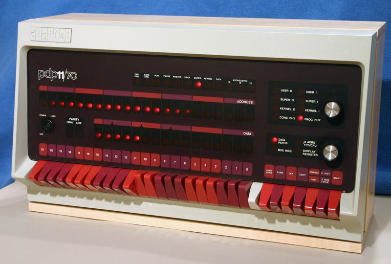
It helped popularize the interactive computing paradigm we take for granted today.