Piper: A Programmable Distributed Training System(developer-blogs.nvidia.com)

Introducing Piper: A Programmable Distributed Training System
TL;DR: New distributed training strategies and optimizations should not require new distributed runtimes.
Large training jobs increasingly combine multiple parallelism strategies such as pipeline, data, and expert parallelism with ZeRO-style sharding, creating placement and GPU scheduling choices that
current frameworks cannot express cleanly.
Today, ML researchers and practitioners choose between building one-off specialized systems that perform well but are hard to adapt, and general-purpose frameworks that are easier to use but expose limited control.
Piper is a user-controllable distributed training system for PyTorch that separates model placement and GPU scheduling from model code and runtime
implementation.
With lightweight model annotations and a small scheduling language, Piper lets users express, visualize, profile, and run high-performance training schedules such as DualPipe-style pipeline- and expert-parallel overlap.

paper: https://arxiv.org/pdf/2606.11169
code: https://github.com/uw-syfi/piper

Composed parallelism dimensions have complex communication patterns

Large model training commonly composes several parallelism dimensions such as:

Data parallelism (DP) replicates model state, runs different data on each replica, and synchronizes gradients with collective communication.
Pipeline parallelism (PP) shards layers into stages and sends activations and gradients between stages with point-to-point communication. Data batches are split into microbatches to keep the pipeline busy.
Expert parallelism (EP) shards the experts in a mixture-of-experts (MoE) layer and routes tokens to and from expert subsets with collective communication.
Tensor parallelism (TP) shards individual tensor operators, such as matrix multiplications, and uses collective communication to assemble partial results.
ZeRO-style sharding reduces redundant optimizer, gradient, and parameter state across DP ranks by sharding model state and introducing additional collective communication to gather and synchronize shards.

Composing parallelism strategies is not one-size-fits-all; the right choice depends on the model architecture, memory constraints, and network topology.
Figure 1 depicts a mixture-of-experts (MoE) model with pipeline parallelism across layers and data/expert parallelism within layers.

Figure 1. A PP x EP x DP placement for a mixture-of-experts model.
Pipeline parallelism places layers across stages, expert parallelism shards expert MLPs, and data parallelism replicates non-expert components like attention.

Composing multiple dimensions creates complex communication patterns and high communication overhead.
A single training step for the Figure 1 placement requires coordinating PP microbatches flowing forwards and backwards through the model, critical-path EP token routing in the forward and backward pass, and DP gradient synchronization.
Thus, maximizing training throughput requires carefully scheduling tensor operators on each GPU to hide communication latency while avoiding bubbles (GPU idle time).

Scheduling tensor operators onto each GPU is hard

MoE training demonstrates the need for fine-grained control over GPU scheduling.
EP adds critical-path all-to-all (A2A) collective communication around expert computation.
DeepSeek-V3 reports that token routing alone produces an approximately 1:1 computation-to-communication ratio in their setup, as experts are distributed across slow inter-node links.
To hide this latency, they introduced the DualPipe schedule, which overlaps expert computation with collective communication from different pipeline-parallel microbatches.
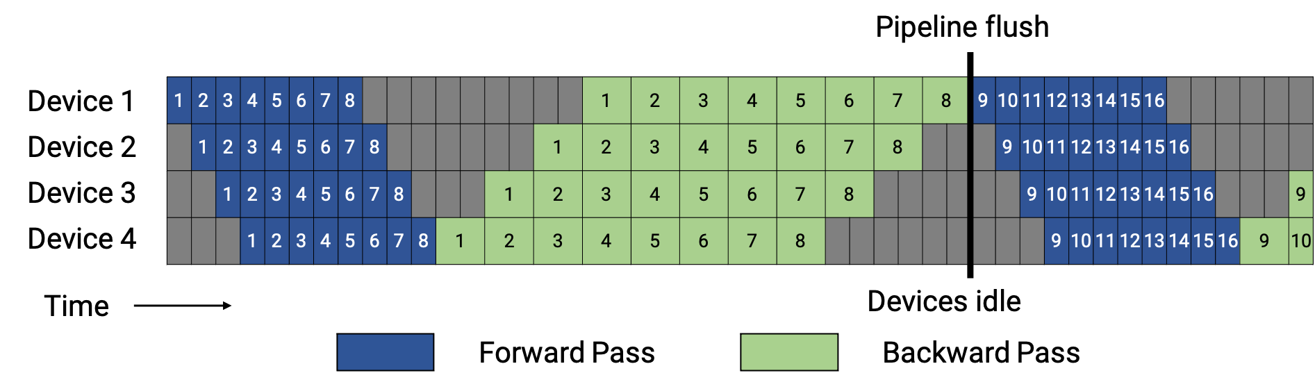
Figure 2 shows a DualPipe schedule variant and highlights an overlapped forward-backward microbatch pair.

Figure 2. DualPipeV schedule for 2-way PP and 4 microbatches.
Numbers are microbatch IDs.
The bolded cells are overlapped forward-backward microbatch pairs.

Scheduling operators onto the GPU is not simple – especially when DP is composed with EP, adding collective all-reduce (AR) communication in the backward pass.
Figure 3 shows different GPU scheduling choices, where streams represent GPU parallelism.

Figure 3. Stream scheduling choices for DP all-reduce and EP all-to-all in an overlapped microbatch pair.
The best choice depends on kernel running times, dispatch ordering, and critical-path dependencies.

Putting A2A and AR on separate streams (a) lets them run concurrently but risks interference on network bandwidth.
Putting A2A and AR on the same stream (b) avoids network interference by serializing the collectives, but can delay communication.
Breaking up the AR into finer-grained units (c) can reduce interference (parameter bucketing is a common example of this strategy), but it’s still hard to predict the overall effect on training throughput, as partitioning can reduce communication efficiency.

Existing general-purpose training frameworks like Megatron, DeepSpeed, and TorchTitan don’t expose low-level scheduling choices.
For example, TorchTitan implements different parallelism dimensions in isolation and eagerly dispatches communication operators for different dimensions on separate streams, in practice supporting only option (a).

As a result, experimenting with choices like (b) or (c) often requires invasive runtime changes
This is because current frameworks lack a central abstraction for flexibly scheduling communication and computation operators across and within GPUs.

Piper’s key idea is to decouple model placement and scheduling choices from both the model implementation and the runtime.
Piper builds abstractions to expose control over inter-device model placement and pipeline schedules as well as intra-device scheduling.

Key idea: Piper decouples model placement and scheduling choices from both the model implementation and the runtime.

Piper at a glance

Piper has two user-facing inputs:

An annotated PyTorch model: standard model code with lightweight tags for schedulable regions such as pipeline stages and MoE experts.
A program of scheduling directives: instructions that tell the Piper compiler how to shard, replicate, order, and overlap those schedulable regions.

Piper’s compiler traces the model using TorchDynamo, extracts annotated regions as schedulable model components, and applies schedule directives as graph rewrites on a distributed training intermediate representation (IR).
The IR is a global training DAG which explicitly encodes compute, communication, data dependencies, temporal dependencies, device placement, and logical stream assignment.

Piper’s runtime then decomposes this global DAG into per-device execution plans and runs them on Ray workers.
Each worker manages local CUDA streams, communicators, model-state buffers, and intermediate tensors.

Figure 4. Piper’s architecture.
The user provides an annotated model and schedule; Piper compiles them into a global training DAG and executes per-worker sub-DAGs with a distributed runtime.

High-performance MoE training with a DualPipe-like schedule in Piper

We will walk through an example of distributing an MoE model with PP x DP x EP placement and a coordinating DualPipe-like training schedule in Piper.
You can run the example yourself with the following command from the Piper repository root after following the setup instructions.

python examples/test_harness.py \
--test-file examples/test_qwen.py \
--base-schedule examples/base-schedules/pp2_dp2_ep2_custom_order.json \
--schedule custom \
--ranks 2 \
--mbs 4 \
--viz

Annotating a Qwen3 MoE model

Piper annotations identify model regions that we will refer to in the user schedule.
For our intended PP x EP x DP placement, we use two tags.

PP_TAG = "PP"
EP_TAG = "EP"

PP identifies pipeline stages and EP identifies expert MLPs inside an MoE layer.
The expert annotation appears inside the AnnotatedMoE module.

class AnnotatedMoE(MoE):
def forward(self, x: torch.Tensor) -> torch.Tensor:
bs, slen, dim = x.shape
x = x.view(-1, dim)

(
top_scores,
selected_experts_indices,
num_tokens_per_expert,
) = self.router(x, self.expert_bias)

(
top_scores_experts_sorted,
token_indices_experts_sorted,
num_tokens_per_expert,
) = self.reorderer(top_scores, selected_experts_indices)

routed_input = x[token_indices_experts_sorted // self.router.top_k]

if self.score_before_experts:
routed_input = (
routed_input.to(torch.float32)
* top_scores_experts_sorted.reshape(-1, 1)
).to(x.dtype)

with piper.annotate(EP_TAG): # Piper annotation
routed_output = self.experts(dispatched_input, num_tokens_per_expert)

gathered_output = gathered_output.reshape(-1, dim)
...

This code wraps the expert computation with piper.annotate(EP_TAG).
The annotation creates a named region that the schedule can later match by filtering on the EP tag.
For example, the filter {"EP": 0} matches the first EP region in the model, {"EP": *} matches all EP regions in the model, and {"EP": -} matches all the non-EP regions in the model.

The pipeline annotation appears in the AnnotatedQwen3TransformerBlock module.

class AnnotatedQwen3TransformerBlock(TransformerBlock):
def __init__(self, config: Qwen3ModelArgs, num_stages: int):
super().__init__(config)
self.num_stages = num_stages

for layer_id in range(config.n_layers):
self.layers[str(layer_id)] = AnnotatedQwen3TransformerBlock(
layer_id, config
)

def forward(
self,
tokens: torch.Tensor,
attention_masks: Optional[AttentionMasksType] = None,
positions: Optional[torch.Tensor] = None,
) -> torch.Tensor:
num_layers = len(self.layers)

for stage_id in range(self.num_stages):
layer_start = stage_id * num_layers // self.num_stages
layer_end = (stage_id + 1) * num_layers // self.num_stages

with piper.annotate(PP_TAG): # Piper annotation
if stage_id == 0:
h = self.tok_embeddings(tokens)

for i in range(layer_start, layer_end):
layer = self.layers[str(i)]
h = layer(h, self.rope_cache, attention_masks, positions)

if stage_id == self.num_stages - 1:
h = self.norm(h)
output = self.output(h)

return output

This wrapper divides the transformer layers into num_stages contiguous ranges and wraps each range with piper.annotate(PP_TAG).
The same model code can therefore be traced with different PP degrees, while Piper assigns stage indices automatically in dataflow order.
Each annotated region becomes a schedulable pipeline chunk.

These annotations are metadata attached during torch.fx tracing.
Piper leverages TorchDynamo to extract an annotated PyTorch operator graph as an fx.Graph.
Piper’s compiler decomposes the graph into sub-graphs per annotated region: these are the smallest schedulable units in our system.

In the next part of the demo, we will see how a user scheduling program instructs Piper’s compiler to shard, replicate, and overlap annotated model regions to build a high-performance distributed training plan.

Scheduling DualPipe-like PP x DP x EP model placement

The second user input is a schedule made up of directives which tell the compiler how to shard, replicate, and overlap annotated model regions.
Internally, each directive encodes a rewrite of the DAG IR that represents the distributed training schedule.

The following directives are snippets from the small example schedule here.
We walk through the JSON directly to explain the interface, but in practice these directives can be generated by schedule builders (described later in this post).

First, we use place to set up the pipeline stages: with data parallelism degree 2, stage 0 runs on devices 0 and 2, and stage 1 runs on devices 1 and 3.

[
{
"op": "place",
"filter": {"PP": 0},
"devices": [0, 2],
"stream": "pp_stream"
},
{
"op": "place",
"filter": {"PP": 1},
"devices": [1, 3],
"stream": "pp_stream"
}
]

When the compiler sees a cross-device data dependency (e.g. from pipeline stage 0 to 1 in the forward pass and stage 1 to 0 in the backward pass), it adds point-to-point send/recv communication nodes to the DAG IR and associates them with a logical stream pp_stream.

A logical stream represents a GPU stream: a work queue whose operations execute in order.
Piper exposes logical streams to identify classes of operations that should be serialized with each other but may overlap with operations on other logical streams when dependencies and hardware resources permit.

Second, we use replicate to tell Piper to synchronize gradients between the two replicas of each pipeline stage.

[
{
"op": "replicate",
"filter": {"PP": 0},
"devices": [0, 2],
"reduce_stream": "dp_stream",
},
{
"op": "replicate",
"filter": {"PP": 1},
"devices": [1, 3],
"reduce_stream": "dp_stream",
}
]

Piper adds collective communication nodes to the DAG IR to synchronize the gradients of replicated model regions after the backward pass.
Piper associates these communication nodes with a logical stream dp_stream.

There are a few optional arguments to replicate.

bucket_size controls communication granularity by bucketing parameters into bucket_size-MB groups. Smaller buckets may expose more overlap or reduce interference, but can also reduce communication efficiency.
shard_grads applies ZeRO-1 gradient sharding to the replicated regions.
shard_params applies ZeRO-2 parameter sharding to the replicated regions. This requires additional collective communication to gather parameter shards before forward and backward computations.
gather_stream allows specifying a separate stream for the gather collectives associated with parameter sharding. This enables finer-grained control over which collectives are overlapped or serialized.

Third, we use shard to split MoE expert regions inside each stage across the stage’s devices and route expert communication on a separate stream.

[
{
"op": "shard",
"filter": {"PP": 0, "EP": "*"},
"devices": [0, 2],
"stream": "ep_stream"
},
{
"op": "shard",
"filter": {"PP": 1, "EP": "*"},
"devices": [1, 3],
"stream": "ep_stream"
}
]

The filter {"PP": 0, "EP": "*"} matches on all expert-annotated chunks inside pipeline stage 0.
Piper adds collective communication to the DAG IR around those expert regions and associates them with the logical stream ep_stream.

Logical streams are a way for the user to control which classes of communication operators are overlappable vs. serialized.
The user does not manually coordinate CUDA streams.
Piper maps logical streams to physical streams and inserts synchronization only when data or temporal dependencies require it.
Through communication bucketing and stream assignment, users can experiment with a range of different low-level scheduling strategies such as those in Figure 3.

Thus far, we have seen how place, replicate, and shard directives describe where computation and communication happen.
For a DualPipe-like schedule, we also need to describe how microbatches of data flow through the pipeline, and how they may overlap.

Scheduling a DualPipe-like pipeline schedule

Piper exposes control over pipeline schedules with split and order directives.
First, we use split to turn each training step into independently scheduled microbatches.

{
"op": "split",
"filter": {},
"dim_name": "MB",
"num_microbatches": 2
}

The empty filter matches the whole training DAG.
Piper duplicates the matched DAG num_microbatches times and tags the copies with MB=0, MB=1, and so on.

order adds temporal dependencies.
Piper provides a PASS tag which supports F (forward), B (backward), BI (backward for inputs), and BW (backward for weights) to refer to different portions of the training DAG.
Backward for inputs vs weights implements ZeroBubble-like backwards pass decomposition.

Second, we use order to encode the pipeline schedule by constraining the order in which microbatch passes run and which may overlap.

[
{
"op": "order",
"filters": [
[{"PP": 0, "MB": 0, "PASS": "F"}],
[{"PP": 0, "MB": 1, "PASS": "F"}],
[{"PP": 0, "MB": 0, "PASS": "B"}],
[{"PP": 0, "MB": 1, "PASS": "B"}]
]
},
{
"op": "order",
"filters": [
[{"PP": 1, "MB": 0, "PASS": "F"}],
[
{"PP": 1, "MB": 1, "PASS": "F"},
{"PP": 1, "MB": 0, "PASS": "B"}
],
[{"PP": 1, "MB": 1, "PASS": "B"}]
]
}
]

The key DualPipe-like construct is the presence of nested filters: it tells Piper that multiple subgraphs can be interleaved to enable intra-device overlapping.
For example, the second filter element of the stage 1 order directive means that microbatch 1 forward and microbatch 0 backward can interleave.

This gives the user control over the schedule structure while leaving mechanical interleaving decisions to the system.
The user says which sub-DAGs may overlap, and Piper decides how to interleave the communication and computation inside that overlappable region.
This is implemented by a compiler pass that decides a total ordering per logical stream: Piper orders compute and communication operators on their respective streams to promote overlapping while avoiding bubbles.

Visualizing the schedule

Piper provides multiple utilities for visualizing distributed training schedules.
The first is a temporal representation of ordering directives, akin to typical pipeline schedule visualizations.
This can help identify unintended pipeline bubbles (white boxes) at a high level.

The simple pipeline schedule from the demo emits the following visualization:

Figure 5. A simple pipeline schedule with 2-way PP, 2 microbatches, and an overlapped forward-backward microbatch pair.

The second utility is a DAG IR visualization.
After applying the scheduling directives and resolving a total ordering per logical stream, Piper produces a visualization of each GPUs local training DAG.
This helps identify how operators will be overlapped on the GPU.

Figure 6. DAG IR snippet for an overlapped forward-backward microbatch pair.

This is a snippet of the PP rank 1 (GPUs 1 and 3) training DAG for our working example.
It shows microbatch 0 backward overlapped with microbatch 1 forward.
Data dependencies are represented by solid lines and temporal dependencies are represented by dotted lines.

The topological order (identified by topo=x) identifies the runtime dispatch order.
Piper uses temporal dependencies to enforce overlapping by constraining total orderings per logical stream (e.g. ep_stream comms all have unique topo index, and the same goes for dp_stream comms).
Runtime scheduling heuristics resolve ambiguous topological ordering across streams by prioritizing SEND > all other nodes > RECV to avoid point-to-point communication interference.

The last visualization utility is custom PyTorch profiler support which combines the profiles for all the PP ranks in each SPMD group and labels the GPU kernels associated with each DAG IR node.
Figure 7 shows the profiler trace for an overlapped forward-backward microbatch on PP rank 1 of our working example.

Figure 7. Profile for an overlapped forward-backward microbatch pair. EP and DP collective communications are completely hidden.

All-to-all kernels on the EP stream and all-reduce kernels on the DP stream are completely overlapped with computation.

Generating directives with schedule-builders

In practice, we don’t expect users to hand-write complete JSON schedules, as they can be verbose for complex pipeline schedules with a high PP degree and number of microbatches.
Instead, we envision that users will write schedule-builders that take in some arguments, such as base schedule with model placement directives, the PP degree, and the number of microbatches, and output a JSON complete with order directives for the desired pipeline schedule.

Schedule builders are ordinary Python functions that emit Piper’s small directive language.
We provide schedule builders for 1F1B, interleaved 1F1B, ZeroBubble, and DualPipeV pipeline schedules.

We hope that researchers will implement new schedule builders to experiment with new inter- and intra-device parallelism strategies.
We imagine the pipeline schedule visualizer will help with visual debugging.
Piper also has safe guards which require order directives to respect the model’s dataflow and device placement.

We will walk through our DualPipeV schedule builder at a high level.

def build_dualpipev_schedule(n_ranks: int, n_mbs: int) -> list[dict]:
if n_mbs < 2 * n_ranks:
raise ValueError(
f"dualpipev requires n_mbs >= 2 * n_ranks, got n_mbs={n_mbs}, "
f"n_ranks={n_ranks}"
)

rows: list[list[_Slot]] = [[] for _ in range(n_ranks)]

for rank in range(n_ranks):
s0 = rank
s1 = 2 * n_ranks - 1 - rank
slots = rows[rank]
counts: dict[tuple[int, str], int] = {}
weight_queue: list[tuple[int, int]] = []

...

return [_order_directive_from_slots(row) for row in rows]

n_ranks is the number of physical PP ranks. n_mbs is the number of microbatches.
For each physical rank, the builder assigns two virtual stages:

s0 = rank
s1 = 2 * n_ranks - 1 - rank

This encodes the V stage placement: each rank owns one stage from the front of the model and one stage from the back.

The builder represents time as a list of slots.
A slot can contain two operations when the schedule permits overlap.
The builder walks through DualPipeV phases: warmup forwards, filling the second virtual stage, main overlapped forward/backward pairs, cooldown backwards, and split backward-weight cleanup:

# Phase 1: F0 warmup.
for _ in range((n_ranks - rank - 1) * 2):
fwd(s0)

# Phase 2: F0F1.
for _ in range(rank + 1):
fwd(s0)
fwd(s1)

# Phase 4: Main overlapped F0B1 + F1B0.
for i in range(n_mbs - n_ranks * 2 + rank + 1):
if i == 0 and rank == n_ranks - 1:
fwd(s0)
full_bwd(s1)
else:
overlap_fb(s0, s1)
overlap_fb(s1, s0)

...

Before returning, _order_directive_from_slots lowers the slot array to the JSON order format.

Run the walkthrough example

A more complete version of the DualPipe-like schedule that we have walked through exists in the repository.
From the Piper repository root:

python examples/test_harness.py \
--test-file examples/test_qwen.py \
--base-schedule examples/base-schedules/pp4_dp2_ep2_v_placement.json \
--schedule dualpipev \
--ranks 2 \
--mbs 4 \
--viz

This command starts from a V-placement base schedule, generates DualPipeV order directives for 2 pipeline ranks and 4 microbatches, runs the Qwen model on the schedule, and writes the generated schedule, schedule visualization, DAG visualization, and throughput/memory statistics under out//.

To collect profiler traces, add:

--pytorch-profiler --pytorch-profiler-iters 3

Evaluation highlights

We compare Piper with Megatron, DeepSpeed, and TorchTitan: asking 3 evaluation questions:

Does Piper perform as well as existing systems on commonly supported strategies?
What benefits in strategy flexibility and performance does Piper provide?
How well does Piper scale?

We will highlight a few results covering question 2, but please see the paper for the full evaluation.

PP x EP and DualPipeV

We evaluate support for DualPipe-like schedules in the baseline systems compared with Piper.
TorchTitan is the only baseline which supports DualPipe-like all-to-all overlapping.

Figure 8. PP x EP throughput for Qwen3 1B and Qwen3 9B with various pipeline schedules.

On Qwen3 1B, Piper-DualPipeV improves throughput by 13% over Piper-1F1B.
TorchTitan-DualPipeV improves only 3% over TorchTitan-1F1B in the same setting.
From brief exploration into the TorchTitan codebase, we attribute TorchTitan’s smaller improvement to unintended serialization between dispatch threads for forward and backward microbatches.

On Qwen3 9B, TorchTitan runs out of memory in the evaluated configuration.
Piper-DualPipeV improves throughput by 10% over Piper’s interleaved 1F1B schedule and 6% over Megatron’s interleaved 1F1B schedule.
Megatron does not support DualPipeV; its interleaved schedule is the closest baseline.
In addition to overlapping EP communication, we plan to further improve performance by integrating Megatron’s optimized kernels.

PP x ZeRO

We evaluate support for composing pipeline parallelism with ZeRO sharding strategies in the baseline systems compared to Piper.
As a quick refresher, ZeRO memory optimizations are successive levels of model state sharding:

ZeRO-1 shards optimizer state.
ZeRO-2 additionally shards gradients.
ZeRO-3 additionally shards parameters.

As the ZeRO level increases, memory savings improve, but the communication overhead grows because model states must be materialized and sharded at the right times.

None of Megatron, DeepSpeed, and TorchTitan fully support pipeline parallelism composed with ZeRO-2 or ZeRO-3.
TorchTitan exposes limited support: we find that model states do not get resharded between all microbatches, so the memory savings are significantly smaller than expected.

We illustrate this in Figure 9, which shows that Piper supports much larger batch sizes by correctly encoding ZeOR-2 and ZeRO-3 sharding semantics.

Figure 9. Peak memory for PP x ZeRO-2 and PP x ZeRO-3 on Qwen3 9B.

Closing

Piper is built around a simple premise: new distributed training strategies should not require new distributed runtimes.

By separating model placement and GPU scheduling from model code and runtime implementation, Piper gives users a concise way to express schedules that would otherwise require invasive framework changes.
We think this makes Piper useful both as a practical training system and as a research platform.

If you are designing a new pipeline schedule, exploring how to overlap communication, or trying to compose parallelism dimensions that current frameworks do not support cleanly, Piper gives you a way to express, visualize, profile, and iterate quickly.
We also hope Piper’s scheduling interface can serve as a useful target for future automatic and agentic scheduling approaches.

Please read our paper and try out the examples in our repository!
We also appreciate feedback.
You can send us an email or leave a GitHub issue.